CEEPR Working Paper
2024-04, March 2024
Sergio Franklin Jr. and
Robert S. Pindyck
Global CO2 emissions are continuing to rise. That may eventually change, but even with a substantial decline in emissions, the atmospheric CO2 concentration will keep growing and remain high for many years. That is why policy objectives have focused on net emissions, and the need to remove CO2 from the atmosphere. But how? Planting trees (afforestation; the practice of establishing forests on land that were not previously forested and reforestation; the practice of reestablishing forest that have been cut down or lost to natural causes) might be seen as an obvious solution, but where and at what cost? Here we focus on forested and forestable land in South America, and use spatially disaggregated data to estimate a supply curve for forest-based atmospheric CO2 removal. The supply curve traces out the marginal cost of removing a metric ton of CO2 as a function of total annual CO2 removal. Each point on the curve corresponds to a specific location, so our analysis tells us where and how many trees can be planted, and at what cost.1
So why don’t we start planting large numbers of trees? Yes, it would take time, but after 10 years or so, net emissions could be substantially reduced. We are indeed planting some trees, but cutting down many more (see Figure 1). From 2015 to 2020, there were about 10 million hectares per year of deforestation, which was partly offset by about 4 million hectares per year of forest gain, for an annual net forest loss of about 6 million hectares. Deforestation occurs because land is valuable, and can be used for agriculture, cattle grazing, mining, and other economic activities.2 And that is one of the main reasons why we are not planting trees in sufficient numbers to have a significant impact on net CO2 emissions. Planting and maintaining trees requires valuable land, which can make it costly.
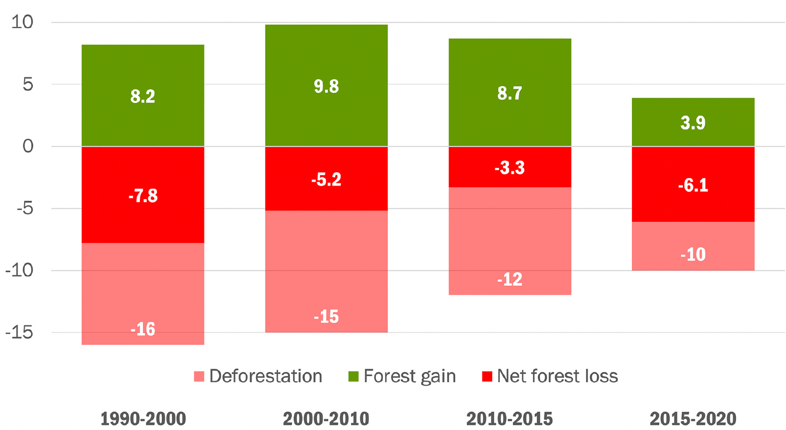
Figure 1. Net Annual Forest Loss.
Source: United Nations’ Food and Agriculture Organization (2020 b) and https://rainforests.mongabay.com/deforestation/
Suppose deforestation at recent rates continues. What impact would an ongoing loss of, say, 6 million hectares per year have for CO2 emissions? Each year CO2 absorption is reduced (i.e., net emissions are increased) by .06 Gt per year, or about 1 Gt after 17 years. But net emissions actually increase by much more, because a tree contains about 200 kg of carbon, which releases around 700 kg of CO2 when the fallen tree decays or (more often) is burned. This in turn implies that an ongoing loss of 6 million hectares per year would increase net CO2 emissions by 0.27 Gt per year, or about 1 Gt after four years.3 Deforestation is a serious problem, but our focus is on forestation. How many hectares can potentially be forested, and at what cost? Macro-level estimates attempt to account for the land that is potentially forestable, but tell us very little about forestation costs, which vary considerably across regions. The variation is due to sharp regional differences in the current use of the land, and in rainfall and other climatic factors that affect forest growth.
We address this problem at the micro level and develop a supply curve for forest-based CO2 removal. The supply curve traces out the marginal cost of removing 1 ton of CO2 from the atmosphere as a function of total annual CO2 removal, all by planting trees. Given data limitations, we focus on forested and forestable areas in South America, which include the Amazon rainforest (accounting for 13 percent of the world’s total forest area), the Atlantic forest, the Gran Chaco region, and areas of savanna and grassland.
We consider planting trees in areas that during the past 50 years were once densely forested but have experienced forest loss, as well as areas that were never forested and may instead have existed as savanna or grassland. Our analysis accounts for the three most important types of cost involved in forestation:
1). Opportunity cost of land. This varies greatly across locations, and is often the largest cost component for forestation. Deforestation occurs because land has economic value, and foresting a hectare of land means it cannot be used for other purposes.
2). Planting and maintenance costs. Planting a tree involves more than sticking an acorn in the ground. It begins with planting and growing seedlings, and then replanting those seedlings with fertilizer, water, and insect repellent. Later, the trees must be protected from insects and pruned as they mature, and sometimes must be replanted. Mature trees have ongoing maintenance costs, which includes continual addition of fertilizer and insect repellent, and depending on the area, water.
3). Forest conservation costs. Later, mature trees must be protected from illegal logging, which is a serious problem in much of the world. Monitoring and law enforcement efforts must be put in place in order to ensure forest conservation.
Based on these costs, we determine where and how many trees can feasibly be planted. We mentioned that water is a critical input; indeed forestation in areas with limited rainfall is usually prohibitively expensive, and most areas deemed suitable for forestation have considerable rainfall. In developing a supply curve for South America, we consider areas where precipitation patterns can potentially support forest growth. The objective is to determine where precipitation patterns make it economical to plant trees and the number of trees that should be planted.
Land opportunity and tree planting costs also vary considerably across regions, as precipitation does. Thus much can be gained by a more micro level approach to the use of forestation for CO2 removal. To show why, Figure 2 below presents one of our main results – a supply curve for forest-based atmospheric CO2 removal in South America. The curve shows the marginal cost of removing (via forestation) one ton of CO2 as a function of total forest-based annual CO2 removal.
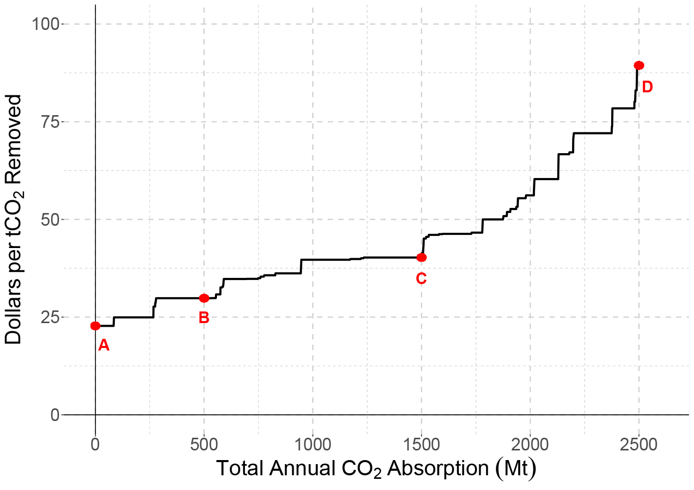
Figure 2. Supply curve for forest-based atmospheric CO2 removal in South America.
The curve shows the marginal cost (in 2020 US dollars) of removing one ton of CO2 per year as a function of
total forest-based CO2 removal. Each point on the curve corresponds to a land grid element.
Point A on the curve shows the lowest cost ($23 per ton) at which CO2can be removed from the atmosphere by planting and maintaining trees in South America. This is the lowest-cost location in part because of plentiful rainfall, but also because of relatively low tree planting and land opportunity costs.4 Point B is also in the Amazon forest of Brazil, state of Para. As at Point A, here rainfall is plentiful, but tree planting costs are higher, so the cost of removing CO2 is $30 per ton. Point C is in the Amazon forest of Brazil, state of Mato Grosso. Land opportunity costs are higher so the cost of removing CO2 is $40 per ton. Finally, Point D, at the top of the curve, is in the Brazilian Cerrado. This area is largely savanna, with lower forestation potential and higher land opportunity costs, so the cost of removing CO2 is about $90 per ton. Figure 2 shows that regional variations in the marginal cost of forestation are large.
We know a single tree can absorb 10 to 40 kg of CO2 per year, depending on climate and the age and type of tree, so to estimate the average CO2 absorption rate for a land grid element, we must account for the variety of trees it contains. We find the total carbon stock accumulation (above and below ground) is 3.0 tons of carbon per hectare per year, or 3.0 × 3.67 = 11 tons of CO2. Given an average tree density of 600 trees per hectare, we estimate the average CO2 absorption rate to be 11,000/600 = 18.333 kg CO2 per tree per year. These estimates apply to trees in tropical moist forests; we use them here because our forestation target zone consists of areas in South America where precipitation patterns are similar to those in tropical forests.
Finally, the cost of planting and maintaining trees is also dependent on the choice of forest recovery technique. Different forest recovery techniques imply different activities and inputs, and thus different costs. “Facilitating natural regeneration” is most economical for land grids with high tree cover (55-65%), “enhancing tree density and enrichening” is frequently used for land grids with medium tree cover (30-55%), typically on the margins of remnant forest areas and in large clearings, and “total planting” is usually most appropriate for land grids with low tree cover (5-30%). Economies of scale make it uneconomical to plant small numbers of trees, so we only consider areas where the forestation potential is at least 10%.
Looking back at Figure 2, each point on the curve shows the cost per ton of CO2 removed for a land grid element in the forestation target zone as a function of total annual CO2 removal. The figure shows that a carbon price at or below $20/tCO2 will have no impact on forest-based CO2 sequestration, a carbon price of $45/tCO2 can induce the sequestration of 1.5 Gt of CO2 per year, and a carbon price of $90/tCO2 can induce the sequestration of 2.5 Gt of CO2 per year. Reductions in agricultural land need not imply higher food prices. Different Brazilian regions and South American countries have different agricultural products, so reductions in agricultural areas can be compensated for by the adoption of best production practices.
Our supply curve applies to only South America, but with sufficient data could be extended to the entire world. If the rest of the world looks like South America (in terms of its potential for forestation), and our supply curve were scaled up accordingly, a considerable amount of CO2 could in principle be removed from the atmosphere via forestation. But doing so would be costly. For example, reducing net CO2 emissions by 25% via forestation would cost something around $1 trillion annually, which is about 1 percent of world GDP.
One could take issue with several aspects of our analysis. First, we have effectively assumed that trees last forever, which is clearly not the case. When trees die, the carbon they have sequestered will be released back into the atmosphere as CO2. Thus, it might seem that planting trees cannot sequester CO2 over the long run because those trees will eventually die. But the key is “eventually.” Trees can live for a few hundred years, so trees planted now will sequester CO2 for many years before those trees will have to be replanted. (Recall that our supply curve is based on a 50-year time horizon.) We have ignored potential demand shifts and innovations in agriculture and in forestry that might occur over the next 50 years. We have also ignored other benefits that forestation can provide, such as water recycling, erosion control, and short-term climate regulation. These benefits have external economic value, and from a public policy perspective should affect the supply curve by reducing the “full” marginal cost of CO2 removal. Lastly, we have not addressed the cost of maintaining existing forest areas, so as to reduce CO2 emissions from deforestation. Because data limitations have limited our analysis to South America, this paper might be viewed as a “proof of concept”.
Further Reading: CEEPR WP 2024-04
Footnotes:
- There is considerable ongoing R&D focused on carbon removal and sequestration (CRS) technologies, but those technologies are currently too expensive for practical use. See Pindyck (2022) and references therein. Other land- and water-based plants, such as mangroves and kelp, can also absorb CO2, but compared to trees, their potential for CO2 absorption is quite limited.
- For a detailed discussion of deforestation in different parts of the world, and recent research to better understand the causes and effects of deforestation, see Balboni et al. (2023).
- 1 kg of carbon is equivalent to 3.67 kg of CO2 because of the two oxygen atoms connected to each carbon atom. Tropical moist forests contain about 130 tons of carbon per hectare above ground (Figure 6 in ForestPlots.net et al. (2021)). To add the belowground biomass, multiply the aboveground carbon stock by 1.26 (Mokany, Raison and Prokushkin, 2006). Tree density is in the range 550-650 trees/ha (ForestPlots.net et al., 2021; Crowther et al., 2015). That leads to the average of 270 kg of carbon per tree. For temperate deciduous and coniferous forests the carbon content is lower, so 200 kg is a conservative average number. See Ramankutty et al. (2007). That CO2 enters the atmosphere fairly quickly, but to measure its impact on temperature, we can “amortize” it over 10 years, so it is roughly equivalent to additional CO2 emissions of 700/10 = 70 kg of CO2 per year. See Amazon Fund (2010) and Franklin and Pindyck (2018). Adding that to the 20 kg of lost absorption yields 90 kg of CO2 per year for each tree cut down, and with an average of 500 trees per hectare this implies an increase in net emissions of 6 × 106 × 500 × .09 = .27 Gt per year.
- There are 160 land grid elements with the same $23 per ton marginal cost spread across 8 Amazon countries. They are all on the short horizontal line that begins at Point A.
About The Authors